Useful Matlab commands

These are some of the commands that I have used in Matlab pretty often. I just put them here for me to have a quick reference. Don't expect any fancy things... :)

t=(0:1/44e3:99999*1/44e3);
osc=sin(2*pi*t*3.9917e+003)';
mixer_out=filter_out.*osc;
bsdelayed=[zeros(25640-13170,1) ;bs];
bsshift=circshift(bs,22800);

figure
subplot(2,1,2)
plot(x,’r’)
clf
hold on
close all  % Closes all figures

filterbuilder
Y=Filter(Hbp,x);

z=amdemod(rx,3.9917e+003,44e3);
fmdemod;
pmdemod;
b=upsample(b,4400); % Insert zeros in between
bs=conv(b,symbol);
abs(fft(rx));

READ WAV FILE
[filename, pathname]=uigetfile('*.wav')
[m d]=wavfinfo(strcat(pathname,filename))
rx = wavread(strcat(pathname,filename));

READ BINARY FILE
[filename, pathname]=uigetfile('.\*.*')  % Open the dialog box
filen=strcat(pathname,filename) % Builds the full file path
fileID = fopen(filen)  % Opens the file and assigns it an ID
A = fread(fileID, inf, 'int16');   % Reads the full file into an Array A, assuming they are 16b integers
plot(A)

% See more http://www.mathworks.com/company/newsletters/articles/Matrix-Indexing-in-MATLAB/matrix.html
v = [16 5 9 4 2 11 7 14];
v(3) % gives 9
v([1 5 6]) % Gives 16, 2, 11
v(3:7) % Gives 9 4 2 11 7

http://www.mathworks.com/support/2014a/matlab/8.3/demos/working-with-arrays-matlab-video.html

Filter design: From Matlab to C code

Note 1:  For this, I am using not only Matlab but the Signal Processing Toolbox. Got to study the other tools that Matlab has to deal with filters...
Note 2: I should write something like this but with some free tool out there... Anyhow, for the moment just use Matlab, as I have it available in my company...

Quick reading, it looks like there are couple of methods:

1. A=ellip(specs) --> H=dfilt.df1(A) where A are the numerator and denominator coeff. This is kind of going analog to then move to digital.
2. D=fdesign.bandpass(specs) --> H=design(D, ellip)

H is the object describing the digital filter (not exactly the coefficients, see more below). We will look in detail and extend the method 2 following Getting started with discrete time filters (dfilt) or fdesign objects.
1/ First got to get the object describing the specification of the filter we want. So, we use fdesign. Just type  "fdesign.bandpass" for a very simple syntax, or go to fdesign for more info.
In our case, we want to create a bandpass filter around 2.5KHz. So, we will do:

>> D=fdesign.bandpass(2000,2200,2800,3000,40,1,40,44100)
And we get:
D =
               Response: 'Bandpass'                     
          Specification: 'Fst1,Fp1,Fp2,Fst2,Ast1,Ap,Ast2'
            Description: {7x1 cell}                     
    NormalizedFrequency: false                          
                     Fs: 44100                          
                 Fstop1: 2000                           
                 Fpass1: 2200                           
                 Fpass2: 2800                           
                 Fstop2: 3000                           
                 Astop1: 40                             
                  Apass: 1                              
                 Astop2: 40

2/ To get the real design, we use:
>> h=design(D,'ellip')
And get:
h =
         FilterStructure: 'Direct-Form II, Second-Order Sections'
              Arithmetic: 'double'                              
               sosMatrix: [4x6 double]                          
             ScaleValues: [5x1 double]                          
     OptimizeScaleValues: true                                  
        PersistentMemory: false
For help, type designmethods(h) to get a list of filters.

3/ At this moment, we may actually like a different structure. Notice it used the default one (direct form II)

but we may want the more standard one. I am going to use direct form I as it is easier for me to identify what output number below matches what coefficient (notice that I am learning while doing this), so, it'll be easier to program:

Note: notice the error on the - sign in the added of b(nb) path.

So, we do:
>> h1  = convert(h,'df1')

h1 =

     FilterStructure: 'Direct-Form I'
          Arithmetic: 'double'      
           Numerator: [1x9 double]  
         Denominator: [1x9 double]  
    PersistentMemory: false

To see what we get, we can do:
>> info(h1)
Discrete-Time IIR Filter (real)   
-------------------------------   
Filter Structure    : Direct-Form I
Numerator Length    : 9           
Denominator Length  : 9           
Stable              : Yes         
Linear Phase        : No

4/ At this point, if we want to see what we got, it is as simple as using the Filter Visualization Tool:
hfvt=fvtool(h1);

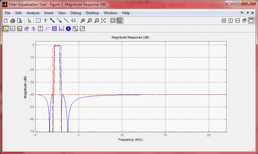
5/ To get the coefficients, use:
num = get(h1,'Numerator');
den = get(h1,'Denominator');

In our case:
num =     0.0099   -0.0729    0.2418   -0.4681    0.5789   -0.4681  0.2418   -0.0729    0.0099
den =     1.0000   -7.4222   24.5776  -47.3746   58.1077  -46.4331  23.6104   -6.9884    0.9229

Where numerator and denominator are (when a0=1, like in our case):

In this kind of structure

Notice that a0 in Matlab is den(1) as the index starts at 1. So, we create in Matlab a piece of code that will do this (equivalent to running y=filter(h1,rx)):

rx2=[zeros(length(num)-1,1);rx];
y=zeros(length(rx)+length(num)-1,1);
for R=length(num):length(rx2)
    data=0;
    for N=1:length(num)
        data=data+rx2(R-N+1)*num(N);
    end
    for D=1:(length(den)-1)
        data=data-y(R-D)*den(D+1);
    end
    y(R)=data/den(1);
end

Translating this into C is straightforward. Notice that the initialization is important. I.e., getting both, input and output past values equal to zero. We can do that adding those in front of our sequences/arrays, or, just make zero the first set of values on those arrays. Of course, this is just for test and assuming you don't care about that data being lost... Either way, you get the point :)
 
The plot on the left is the result using "filter" while the one on the right is the one from the "C" code.

Other useful information:

For an automatic way to do it: Forum describing how to do it
From Simulink to C
From Matlab to HDL
Real Time Workshop Embedded Coder

Matlab filter design
Designing Low Pass FIR filters
FDATool

To use your filter (DUH!): y=filter(num,den,x);
To see the impulse response of your filter use [h,t] = impz(num,den) and plot(t,h)
To check if it is stable: isstable(h) - Note: I didn't get it to work where I can check it with filter running in a given precision

Nice write up on filter theory: http://www.mikroe.com/chapters/view/73/chapter-3-iir-filters/
And another one...
And one more!

Installing Matlab (exclusive for my company)

This works with my company, so, may not work with yours...

1. Go to: http://flames.design.**.com/ReleaseMessages/mathworks/relmsg_mathworks_R2011b.html, where ** should be replaced by the name of my company.
2. Follow those instructions.
3. To add a toolbox follow also those instructions. It is missing that you will have to re-run the installer again if you did it at a different time. Going through control panel does not work:
4. You have to do like if you were going to install a brand new matlab but choose "custom". 
5. If the zip files of the toolboxes are on the same directory as the installer, it will detect those and list them here. 
6. Select them and install... 
7. It may give you an error that the installation may not be all right, in the end, but ignore it.
8. Run Matlab and you should see those packages after typing "ver"
9. You should be able to run also now the functions on those toolboxes.
10. To change where you want it to start by default use, for instance: userpath('C:\MATLAB\work')

Enjoy! :)